Efficient, practical super resolution in the browser

If you are a regular user who just wants to know how this app works (e.g. why is it free? Is this legit?) without getting into code or math, you can read the other page I wrote.

This article is essentially a self-published technical article explaining how this open source utility was built, including details on AI model development and implementation.

Background

free.upscaler.video is an open source utility to improve the image quality of videos and images. It runs entirely within the browser, using neural networks written as shaders in WebGPU and WebGL, and a Web API called WebCodecs to handle video processing.

This enables users to enhance the quality of images and videos for free without installing or configuring software, requiring logins, uploading videos or signup. As of January 2026, approximately 120,000 users visit the tool every month without any promotion.

I built this tool as a learning exercise in December 2023 to practice writing neural networks in WebGPU and had no expectation that it would actually be used by anyone.

The Neural Networks

Image/Video quality enhancement is accomplished via super resolution, a well established technique for the purpose.

Prior Work

Established Research

Most of the established literature in super resolution and image restoration more generally, from VDSR [1] (2015) to ESRGAN [2] (2018) to SR3 [3] (2021) to SwinSR [4] (2022), focuses on novel architectures while optimizing for industry-standard benchmarks like SSIM and PSNR on established academic datasets like DIV2K. RealESRGAN [5] (2021) was notable in focusing primarily on dataset augmentation and real-world use cases, and to this day remains the most popular open source model for generic, user-facing image & video quality enhancement. None of the established research focuses on how models are actually deployed for real world inference, with a CUDA runtime taken as a universal given. Academic datasets and benchmarks also don’t really correspond to what actual real world users are looking for when searching for image or video enhancement software.

Open Source Projects

Open Source projects like Video2x [6] (2018) and Anime4K [7] (2019) have bridged the gap between academia and actual users to some extent, with the former packaging existing models like RealESRGAN into a video-processing desktop utility. Anime4K was notable for developing CNN based neural networks, written as OpenGL shaders to use within video player software for real-time super-resolution on devices without a cuda runtime or discrete graphics cards.

The actual problem

A key limitation for most of the established research is that academics don’t really consider what average, ordinary users searching for video or image enhancement are actually looking for. While it hardly counts as a rigorous academic study, an anonymous, opt-in survey of users of this website (free.upscaler.video) with 173 responses collected in March 2024 indicated the top categories of video content users were looking to improve:

Content type	Responses	Percentage
AI generated videos	81	46.0%
Downloaded or torrented movies	46	26.5%
Video Camera, Smartphone or Drone footage	24	13.9%

Keep in mind that this was a small sample size with an opt-in survey, taken from users visiting “free.upscaler.video” so there are all sorts of potential biases.

Nevertheless, the most common use case essentially boils down to the fact that free AI video generation tools output video at resolutions between 480p and 720p, and marketers and/or content creators are looking for a free/quick way to improve the quality to 1080p or 4K.

Very few ordinary users actually have NVIDIA GPUs with CUDA installed and configured, and at current GPU prices, almost all the models discussed in established research would result in inference costs of ~$100 USD to $1000 USD per hour of video content, which is orders of magnitude higher than what most ordinary users would be willing to pay.

For the most common use cases from ordinary users searching for image/video quality enhancement on search engines, almost all the established academic research is functionally useless and irrelevant.

WebGPU/WebGL & WebNN

For most research, the focus is on architecture and training strategy, with the deployment environment given little to no thought (most papers just assume a cuda runtime). When there is thought put into inference, for example with MobileNetV2, it is primarily focused on adjusting the architecture to reduce parameter count or floating point operations in general.

The problem with that is that, while parameter count and flops enable pure mathematical comparisons between models and sure, more flops leads to longer inference times, there are so many implementation details that actually determine inference runtime that are independent of architecture.

Neural network runtime environments for client-side inference, like TFLite or ONNX.js are incredibly inefficient. I surmise that the reason is overhead from the need to port server-side general purpose runtimes like TensorFlow and Onnx to the client.

Whatever the reason, I’ve developed a number of neural networks, including MobileNetV2, EfficientNet and VDSR, directly as shaders for WebGL and WebGPU, and I’ve found the shader implementations to be 2.5x to 30x faster than equivalent TFLite equivalents [8]:

Model	Input	WebGL	TFLite (SIMD)	Speedup
MobileNetV2	Per frame	4 ms	10 ms	2.5x
VDSR (100k params)	360p image	30 ms	1000 ms	33x

I’ve also found that the performance difference is bigger for simpler architectures (like VDSR, which is almost entirely Conv2d + ReLU), not only when writing as shaders for OpenGL/WebGL/WebGPU, but also when using TensorRT on the server and neural-network specific hardware acceleration environments like CoreML for Apple Silicon.

For efficient client-side inference, it is therefore imperative to understand the inference environment, and the particulars specifically of WebGL and WebGPU. You need to design architecture around the specifics of WebGL and WebGPU.

WebGL and WebGPU are browser APIs that enable hardware-accelerated computation via the user’s graphics card, whether integrated or dedicated. WebGL is primarily a graphics programming language that could be adapted for neural network inference with some work, whereas WebGPU is a newer, more general purpose API that also facilitates general purpose hardware-accelerated computation.

WebNN enables direct access to dedicated neural network accelerators like the Neural Engine on Apple Silicon, but defaults to TensorFlow-based inference when no neural engine is present, which as we saw is much slower than native WebGL/WebGPU shaders.

As of January 2026, WebNN also has no efficient way to directly read from and write to graphics memory (though there is a W3C proposal to address this), which means the vast majority of computation involved in running these models would be consumed by buffer copies rather than the actual neural network inference, making WebNN not a useful inference engine for the stated use case.

WebGL shaders

The most expensive and time-consuming parts of end-to-end inference isn’t actually the number of floating point operations, it is buffer read/write operations.

While WebGPU is more flexible than WebGL on this, WebGPU is still not fully supported everywhere, with ~78% global support [9], so we need to design around the particulars of WebGL which is far more supported at 96% global support [10].

If you have a background in training neural networks you’d be accustomed to tensors and how they flow through the model. WebGL is a graphics programming language and doesn’t care about tensors.

Instead, your base operating unit is a Texture, which is basically a 4-channel image with a height and width. WebGL works by defining a Fragment shader, which is an individual function that you can run on every single pixel of a source image.

Within a single execution of a shader, you can read from up to 8 textures at a time, but you can only write to 1 texture.

This system was designed for graphics processing, and so one simple operation that an AI researcher and a graphics processor can both understand is a simple gaussian blur operation, which is just a conv2d with a fixed gaussian kernel:

#version 300 es
precision highp float;

in vec2 v_texCoord;
out vec4 outColor;

uniform sampler2D u_image;
uniform vec2 u_imageSize;

void main() {
    // Gaussian 3x3 kernel weights
    float kernel[9] = float[9](
        1.0/16.0, 2.0/16.0, 1.0/16.0,
        2.0/16.0, 4.0/16.0, 2.0/16.0,
        1.0/16.0, 2.0/16.0, 1.0/16.0
    );

    // 3x3 convolution offsets
    vec2 offsets[9] = vec2[9](
        vec2(-1.0, -1.0), vec2(0.0, -1.0), vec2(1.0, -1.0),
        vec2(-1.0,  0.0), vec2(0.0,  0.0), vec2(1.0,  0.0),
        vec2(-1.0,  1.0), vec2(0.0,  1.0), vec2(1.0,  1.0)
    );

    vec4 result = vec4(0.0);
    ivec2 pixelCoord = ivec2(v_texCoord * u_imageSize);

    // Apply convolution kernel to each neighboring pixel
    for (int i = 0; i < 9; i++) {
        ivec2 sampleCoord = pixelCoord + ivec2(offsets[i]);
        vec4 sample = texelFetch(u_image, sampleCoord, 0);
        result += sample * kernel[i];
    }

    outColor = result;
}

While adapting this runtime to general neural network operations might be conceptually difficult, if all you are doing is super resolution where most of the computation is done with image tensors of the same height and width as the source image, you can start to see how you could adapt this to a convolutional neural network.

If you have an image tensor of height × width × num_channels, you can split your tensor among multiple textures. You can represent a height × width × 8 tensor as 2 textures of height × width, with each texture having 4 channels.

If you want an operation to read in a H × W × 8 channel tensor, and write out to an H × W × 8 channel tensor (a simple conv2d layer), you would read in two textures, and write to the output tensor 2 times, first writing to the first 4 channels, and then again writing to the last 4 channels because you can only write out to 1 texture at a time.

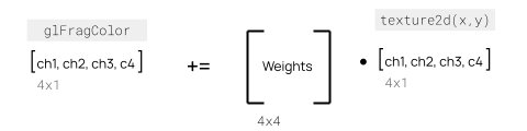
To actually do the conv2d calculation, you need to apply the conv2d kernel at each pixel position. You can read the pixel value of a texture at any given location using texture2D(x, y) which gives a 4-channel array, meaning you can only read in 4 channels of an image tensor at a time.

You can also only write out to 4 channels at a time. By far the most efficient way to implement this is to format your weights in such a way that you can reduce all computations down to a set of kernel weights being read as a 4 × 4 matrix, multiplied by the 4-channel texture, and written out to a 4-channel texture.

Here’s an example showing a conv2d layer with 8 input channels (2 textures) writing to 4 output channels (1 texture) with ReLU activation:

#version 300 es
precision highp float;

in vec2 v_texCoord;
out vec4 outColor;

uniform sampler2D u_input0;  // First 4 channels
uniform sampler2D u_input1;  // Next 4 channels
uniform vec2 u_inputSize;

// Weights: 9 kernel positions × 8 input channels × 4 output channels
// Organized as mat4 for efficient 4-channel operations
uniform mat4 u_kernels[18];  // 9 positions × 2 textures (8 input channels)
uniform vec4 u_bias;

void main() {
    // 3×3 convolution offsets
    vec2 offsets[9] = vec2[9](
        vec2(-1.0, -1.0), vec2(0.0, -1.0), vec2(1.0, -1.0),
        vec2(-1.0,  0.0), vec2(0.0,  0.0), vec2(1.0,  0.0),
        vec2(-1.0,  1.0), vec2(0.0,  1.0), vec2(1.0,  1.0)
    );

    vec4 result = vec4(0.0);
    ivec2 pixelCoord = ivec2(v_texCoord * u_inputSize);

    // Apply convolution across all 8 input channels
    for (int i = 0; i < 9; i++) {
        ivec2 sampleCoord = pixelCoord + ivec2(offsets[i]);

        // Read 4 channels from first texture
        vec4 input0 = texelFetch(u_input0, sampleCoord, 0);
        result += u_kernels[i] * input0;

        // Read 4 channels from second texture
        vec4 input1 = texelFetch(u_input1, sampleCoord, 0);
        result += u_kernels[i + 9] * input1;
    }

    // Add bias and apply ReLU activation
    result += u_bias;
    outColor = max(result, vec4(0.0));
}

An even more efficient optimization is to use CReLU instead of ReLU. With CReLU, each input channel effectively becomes two channels - one for positive activations max(x, 0) and one for negative activations max(-x, 0). This means a single 4-channel texture read can yield 8 effective channels, doubling your network’s representational capacity without additional memory bandwidth:

#version 300 es
precision highp float;

in vec2 v_texCoord;
out vec4 outColor;

uniform sampler2D u_input0;
uniform sampler2D u_input1;
uniform vec2 u_inputSize;
uniform mat4 u_kernels[36];  // 9 positions × 4 CReLU variants (pos/neg × 2 textures)
uniform vec4 u_bias;

void main() {
    // 3×3 convolution offsets
    vec2 offsets[9] = vec2[9](
        vec2(-1.0, -1.0), vec2(-1.0, 0.0), vec2(-1.0, 1.0),
        vec2(0.0, -1.0),  vec2(0.0, 0.0),  vec2(0.0, 1.0),
        vec2(1.0, -1.0),  vec2(1.0, 0.0),  vec2(1.0, 1.0)
    );

    vec4 result = vec4(0.0);
    ivec2 pixelCoord = ivec2(v_texCoord * u_inputSize);

    // Process both inputs with CReLU
    for (int i = 0; i < 9; i++) {
        ivec2 sampleCoord = pixelCoord + ivec2(offsets[i]);

        vec4 pix0 = texelFetch(u_input0, sampleCoord, 0);
        vec4 pix1 = texelFetch(u_input1, sampleCoord, 0);

        // CReLU: positive parts
        result += u_kernels[i] * max(pix0, vec4(0.0));
        result += u_kernels[i + 9] * max(pix1, vec4(0.0));

        // CReLU: negative parts
        result += u_kernels[i + 18] * max(-pix0, vec4(0.0));
        result += u_kernels[i + 27] * max(-pix1, vec4(0.0));
    }

    result += u_bias;
    outColor = result;
}

Understanding these particulars of the inference environment (WebGL in this case) leads to clear architectural choices for the most efficient inference:

• Stick to Conv2d - Avoid operations that don’t map cleanly to texture operations
• Use channel counts that are multiples of 4 - Aligns with 4-channel texture format
• Use CReLU instead of ReLU - Doubles effective channel count without additional memory bandwidth

Architecture

Working backwards from those limitations, I therefore devices the architecture as a simple 2x upscaler with a highway depth of n (a multiple of 4), and a number of layers

from tensorflow.keras.initializers import RandomNormal
import tensorflow.keras.backend as K

def SRModel( input_depth=3, highway_depth=4, block_depth=4, init='he_normal', init_last = RandomNormal(mean=0.0, stddev=0.001)):

    input_shape = [None, None, input_depth]
    input_lr = tf.keras.layers.Input(shape=input_shape)
    input_lr2 = tf.keras.layers.UpSampling2D(size=(2, 2), interpolation='bilinear')(input_lr)
   
    x = input_lr
    for i in range(block_depth):
        x = tf.keras.layers.Conv2D(highway_depth, (3, 3), padding='same', kernel_initializer=init)(x)
        x = tf.nn.crelu(x)
    
    x = tf.keras.layers.Conv2D(highway_depth, (3, 3), padding='same', name="conv2d_last",  kernel_initializer=init)(x)
    x = PixelShuffle(4)(x)
    x = tf.keras.layers.Add()([x, input_lr2])
    model = tf.keras.models.Model(input_lr, x)
    return model

Where the pixels shuffle layer was modified from the built-in version to facilitate shader generation

class PixelShuffle(tf.keras.layers.Layer):
    def __init__(self, input_depth, **kwargs):
    super(PixelShuffle, self).__init__(**kwargs)
    self.input_depth = input_depth
    
        def build(self, input_shape):
            super(PixelShuffle, self).build(input_shape)
    
        def call(self, x):
            x = tf.split(x, (self.input_depth // 4), axis=-1)
            return tf.concat([tf.nn.depth_to_space(xx, 2) for xx in x], axis=-1)

Dataset

The training dataset was constructed from five distinct categories to ensure broad coverage of real-world use cases:

Category	Source	Resolution	Processing
Faces	FFHQ [11]	512×512	Random patch extraction
Natural Images	DIV2K [12]	512×512	Random patch extraction
Animation	Synla+	512×512	Native resolution
Synthetic UI	Custom-generated	512×512	Procedurally rendered (simulating screenshares)
AI-Generated	Stable Diffusion 2.0	512×512	4 patches extracted per 1024×1024 generation

The synthetic UI category was designed to improve performance on screenshots and screen recordings, a common use case identified in the user survey. Images were procedurally generated using scripts to create synthetic user interface elements, charts, and text overlays typical of screen capture content.

For the AI-generated category, prompts were generated using a custom script to ensure diversity across subjects, styles, and compositions. Each Stable Diffusion 2.0 output (1024×1024) was divided into four non-overlapping 512×512 patches to maximize data efficiency.

The final dataset consisted of 50,000 total patches (10,000 from each category). For categories with more available data than required, patches were randomly sampled to reach the target count. This balanced approach ensured equal representation across all five categories.

All patches were standardized to 512×512 resolution for consistent training. The training strategy employed a two-phase approach: models were first trained for 6 epochs on a randomly shuffled mix of the entire dataset, followed by 6 epochs of specialized training on a specific content category. This curriculum learning approach produced category-specific models optimized for faces, natural images, animation, synthetic UI, or AI-generated content.

Dataset augmentation proved critical to model performance. Following the approach established in RealESRGAN [5], the primary degradation pipeline focused on simulating real-world compression artifacts rather than simple downsampling. JPEG compression simulation and ring blur artifacts were essential, as the practical goal of “quality enhancement” predominantly involves correcting compression artifacts rather than pure super-resolution.

def augment_images(img):
    img = img / 255

    img = tf.image.random_hue(img, 0.5)
    img = tf.image.random_contrast(img, 0.5, 2.0)
    img = tf.clip_by_value(img, 0, 1)
    
    img = tf.image.random_flip_left_right(img)
    img = tf.image.rot90(img, k=tf.experimental.numpy.random.randint(4, dtype=tf.int32))

    if tf.random.uniform(shape=()) < 0.1:
        img = degrade_blur_gaussian(img, 1.0, shape=(5, 5))

    lr, hr = img, img

    if tf.random.uniform(shape=()) < 0.1:
        random_sigma = tf.random.uniform(shape=(), minval=2.0, maxval=5.0)
        lr = degrade_ring(lr, random_sigma, shape=(5, 5))

    if tf.random.uniform(shape=()) < 0.1:
        random_sigma = tf.random.uniform(shape=(), minval=0.1, maxval=0.5)
        lr = degrade_blur_gaussian(lr, random_sigma, shape=(3, 3))

    hr_shape = tf.shape(hr)
    if tf.random.uniform(shape=()) < 0.5:
        lr = tf.image.resize(lr, [hr_shape[-3]//2, hr_shape[-2]//2], method="area")
    else:
        lr = tf.image.resize(lr, [hr_shape[-3]//2, hr_shape[-2]//2], method="bicubic")

    if tf.random.uniform(shape=()) < 0.8:
        lr = degrade_rgb_to_yuv(lr, jpeg_factor=tf.experimental.numpy.random.randint(70, 90, dtype=tf.int32), chroma_subsampling=True, chroma_method="area")
        lr = degrade_yuv_to_rgb(lr, chroma_method="bicubic")
        #Process hr alongside with lr to prevent mean shift from jpeg and conversion errors
        hr = degrade_rgb_to_yuv(hr, jpeg_factor=95, chroma_subsampling=False)
        hr = degrade_yuv_to_rgb(hr)

    return lr, hr

Training

Three model variants were trained to provide different speed/quality tradeoffs:

Model Size	Highway Depth	Layers	Parameters	Target Use Case
Small	8 channels	7	~10k	Real-time, mobile devices
Medium	16 channels	7	~30k	Balanced performance
Large	28 channels	7	~100k	Maximum quality

Each configuration was trained using the two-phase curriculum approach: 6 epochs on the mixed dataset followed by 6 epochs on category-specific data, yielding 15 total models (3 sizes × 5 content categories).

The learning rate was manually scheduled, decreasing gradually from 1e-4 to 1e-5 over the training duration to ensure stable convergence.

Model Deployment: TensorFlow to WebGL Shaders

The most technically challenging aspect of the implementation is translating trained TensorFlow models into WebGL/WebGPU shaders. Unlike standard deployment workflows (TFLite, ONNX), this requires complete manual translation of weights and operations.

Weight Restructuring

TensorFlow stores Conv2d weights as [kernel_height, kernel_width, input_channels, output_channels]. For efficient shader execution, these must be restructured into mat4 uniforms that process 4 channels at once. For a 3×3 Conv2d layer with 8 input channels and 4 output channels:

• TensorFlow shape: [3, 3, 8, 4] = 288 weights
• Shader format: 18 mat4 uniforms (9 kernel positions × 2 input textures)
• Each mat4 represents: 4 input channels → 4 output channels transformation

The weight export script [22] performs this restructuring:

# Actual weight restructuring from export script
def reshape_for_shader(weights):
    # weights shape: [kernel_h, kernel_w, input_channels, output_channels]
    kernel_h, kernel_w, in_channels, out_channels = weights.shape

    flattened_weights = []

    # Process input channels in 4-channel chunks (for input textures)
    for in_start in range(0, in_channels, 4):
        in_end = min(in_start + 4, in_channels)

        # Iterate spatial positions in column-major order (x then y)
        for kx in range(kernel_w):
            for ky in range(kernel_h):
                # Create 4×4 matrix (WebGPU mat4)
                weight_matrix = np.zeros((4, 4))

                # Fill with actual weights (padded to 4×4)
                actual_in = in_end - in_start
                actual_out = min(4, out_channels)
                weight_matrix[:actual_in, :actual_out] = \
                    weights[ky, kx, in_start:in_end, :actual_out]

                # Flatten and append
                flattened_weights.extend(weight_matrix.flatten())

    return flattened_weights

Implementation References

The complete implementation involves three components:

1. Network definition [23] - Shader-based neural network architecture
2. Layer implementations [24] - Individual shader layer code (Conv2d, CReLU, PixelShuffle)
3. Export script [22] - TensorFlow weight extraction and restructuring

This manual translation process is labor-intensive but necessary to achieve the 2.5-33× speedup over TFLite observed earlier. Automated tools like ONNX.js cannot perform the weight restructuring optimizations required for efficient WebGL execution.

Performance

Absolute SSIM scores are not meaningful without specifying the degradation pipeline. For the DIV2K validation set using the augmentation pipeline described above, the models achieved the following SSIM improvements:

Model	Parameters	SSIM Improvement	Inference Speed (M4 MacBook Pro, WebGPU)
Small	~10k	+6.4 points	120 FPS @ 720p
Medium	~30k	+8.2 points	40 FPS @ 720p
Large	~100k	+9.3 points	15 FPS @ 720p

On modest graphics cards like the one on my $200 Chromebook, the small model still achieves 40 FPS on integrated graphics demonstrates the effectiveness of the WebGL-optimized architecture. These speeds enabled real-time preview during video processing, significantly improving user experience compared to offline batch processing workflows.

Video Processing Pipeline

The video upscaling implementation follows a streaming architecture using WebCodecs [13] and the Streams API to process videos without loading entire files into memory.

Architecture Overview

The pipeline consists of five stages:

1. Demuxing - Extract encoded video chunks from container format
2. Decoding - Convert EncodedVideoChunk → VideoFrame using VideoDecoder
3. Processing - Apply AI upscaling via WebGPU shaders to each frame
4. Encoding - Convert processed VideoFrame → EncodedVideoChunk using VideoEncoder
5. Muxing - Write encoded chunks to output container

Implementation

The implementation uses MediaBunny [14] as the primary demuxing/muxing library, which provides a high-level API over WebCodecs while handling the complexity of container formats, timestamp management, and audio synchronization.

// Simplified pipeline structure
const pipeline = {
  demuxer: new MediaBunny.Demuxer(inputFile),
  decoder: new VideoDecoder(config),
  renderer: new WebSR.Processor(modelWeights),  // WebGPU upscaling
  encoder: new VideoEncoder(outputConfig),
  muxer: new MediaBunny.Muxer(outputHandle)
};

Backpressure Management

Critical to performance is managing backpressure across the pipeline stages. The implementation limits:

• Decode queue: Maximum 20 chunks to prevent decoder overflow
• Active frames: Maximum 10 VideoFrame objects in memory
• Encode queue: Maximum 20 frames to prevent encoder overflow
• Chunk buffering: Throttled file reading based on downstream capacity

The browser’s Streams API automatically handles backpressure propagation—when encoding slows down, decoding automatically throttles, which in turn slows file reading. This prevents memory exhaustion while maximizing throughput.

Audio Handling

Audio is passed through without re-encoding to preserve quality and avoid sync issues. The original EncodedAudioChunk objects are copied directly from the input demuxer to the output muxer, maintaining perfect audio/video synchronization via timestamp preservation.

File System Access

The implementation leverages the File System Access API [15] to write directly to disk, avoiding the 2GB blob size limit in some browsers. When File System Access is unavailable (Firefox, older browsers), it falls back to in-memory ArrayBuffer storage with a download trigger.

Progress Tracking

Real-time progress estimation is achieved by:

1. Tracking total frames from demuxer metadata
2. Counting encoded frames completed
3. Measuring time per frame (exponential moving average)
4. Calculating estimated time remaining: (remainingFrames × avgTimePerFrame)

The WebGPU rendering pipeline enables real-time preview by drawing both original and upscaled frames to separate canvases at 30 FPS, providing immediate visual feedback during the multi-minute encoding process.

Impact & Adoption

Since launching in December 2023, free.upscaler.video has demonstrated the viability of browser-based AI video processing at scale:

Usage Metrics

• ~4,000 daily users with 20% bounce rate
• 5-minute average session duration (significantly above typical web app engagement)
• ~100 hours of video processed daily (median video length: 1 minute)
• Zero server infrastructure costs - all processing runs client-side

Hardware Compatibility

Real-world usage spans diverse hardware configurations, validating the WebGL-first architecture:

Hardware Class	Example Device	Performance (Small Model)
High-end Desktop	Apple M4 MacBook Pro	120 FPS @ 720p
Mid-range Desktop	Integrated GPU systems	40-60 FPS @ 720p
Budget Chromebook	$200 Chromebook	40 FPS @ 720p
Modern Mobile	Recent Android/iOS	15-30 FPS @ 720p

The 20% bounce rate (vs. 50-70% typical for web utilities) suggests users successfully complete their processing tasks, indicating the implementation handles edge cases and diverse video formats reliably.

Ecosystem Contribution

The codec compatibility testing embedded in the tool has contributed 45.5M+ codec tests across 143K+ user sessions to webcodecsfundamentals.org [20], providing the community with real-world WebCodecs support data across browsers and platforms. The complete dataset and codec support tables are publicly available [21].

This validates WebCodecs and WebGPU as production-ready APIs for compute-intensive applications, not just demos or prototypes.

Open Source Implementation

The complete implementation is available as open source:

• WebSR Library [16] - Core WebGL/WebGPU super-resolution engine with shader implementations
• Custom Training [17] - TensorFlow training scripts and dataset augmentation pipeline
• NPM Package [18] - @websr/websr for integrating AI upscaling into web applications
• Free Upscaler Website [19] - Complete video upscaling application source code

Developers can integrate the upscaling models into their own applications via the npm package, train custom models using the provided training scripts, or fork the entire video upscaling implementation.

References

[1] Kim, J., Lee, J. K., & Lee, K. M. (2016). Accurate image super-resolution using very deep convolutional networks. Proceedings of the IEEE conference on computer vision and pattern recognition, 1646-1654.

[2] Wang, X., Yu, K., Wu, S., Gu, J., Liu, Y., Dong, C., … & Change Loy, C. (2018). Esrgan: Enhanced super-resolution generative adversarial networks. Proceedings of the European Conference on Computer Vision (ECCV) Workshops.

[3] Saharia, C., Ho, J., Chan, W., Salimans, T., Fleet, D. J., & Norouzi, M. (2021). Image super-resolution via iterative refinement. arXiv preprint arXiv:2104.07636.

[4] Conde, M. V., Choi, U. J., Burchi, M., & Timofte, R. (2022). Swin2SR: SwinV2 Transformer for Compressed Image Super-Resolution and Restoration. European Conference on Computer Vision, 669-687.

[5] Wang, X., Xie, L., Dong, C., & Shan, Y. (2021). Real-ESRGAN: Training Real-World Blind Super-Resolution with Pure Synthetic Data. Proceedings of the IEEE/CVF International Conference on Computer Vision, 1905-1914.

[6] Video2X. (2018). GitHub repository. https://github.com/k4yt3x/video2x

[7] Anime4K. (2019). GitHub repository. https://github.com/bloc97/Anime4K

[8] Bhattacharyya, S. (2020). Building a More Efficient Background Segmentation Model Than Google. Medium. https://medium.com/vectorly/building-a-more-efficient-background-segmentation-model-than-google-74ecd17392d5

[9] WebGPU browser support. Can I use. https://caniuse.com/webgpu (accessed January 2026)

[10] WebGL 2.0 browser support. Can I use. https://caniuse.com/webgl2 (accessed January 2026)

[11] Karras, T., Laine, S., & Aila, T. (2019). A style-based generator architecture for generative adversarial networks. Proceedings of the IEEE/CVF conference on computer vision and pattern recognition, 4401-4410.

[12] Agustsson, E., & Timofte, R. (2017). NTIRE 2017 Challenge on Single Image Super-Resolution: Dataset and Study. Proceedings of the IEEE Conference on Computer Vision and Pattern Recognition Workshops, 126-135.

[13] WebCodecs API. W3C Working Draft. https://www.w3.org/TR/webcodecs/

[14] MediaBunny. npm package. https://www.npmjs.com/package/mediabunny

[15] File System Access API. MDN Web Docs. https://developer.mozilla.org/en-US/docs/Web/API/File_System_Access_API

[16] WebSR - Browser-based Super Resolution. GitHub repository. https://github.com/sb2702/websr/

[17] WebSR Custom Training Scripts. GitHub repository. https://github.com/sb2702/websr/tree/main/custom_training

[18] @websr/websr. npm package. https://www.npmjs.com/package/@websr/websr

[19] Free AI Video Upscaler - Source Code. GitHub repository. https://github.com/sb2702/free-ai-video-upscaler

[20] WebCodecs Fundamentals - Codec Support Dataset. https://webcodecsfundamentals.org/datasets/codec-support/

[21] WebCodecs Codec Support Table. https://webcodecsfundamentals.org/datasets/codec-support-table/

[22] WebSR TensorFlow to WebGPU Export Script. GitHub. https://github.com/sb2702/websr/blob/main/custom_training/direct_webgpu_export.py

[23] WebSR Network Architecture Implementation. GitHub. https://github.com/sb2702/websr/blob/main/src/networks/anime4k/cnn-2x-l.ts

[24] WebSR Shader Layer Implementations. GitHub. https://github.com/sb2702/websr/blob/main/src/layers/anime4k/conv2d-8x4.ts